A simple approach for multivariate
wavelets are tensor products of univariate multiscale functions.
There are two different methodologies. In the first case, the univariate
functions for the different coordinate directions have the same level of
refinement. This leads to essentially isotropic basis functions.
In the second case, there is no restriction on the refinement level.
The tensor product approach is used in a straight forward manner and the
wavelets are defined by
 Depending on how much the level indices for
the various coordinate directions differ, one ends up with
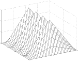
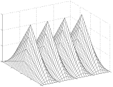
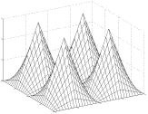
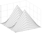
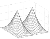
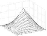
isotropic as well as strongly anisotropic basis functions. Some examples
are shown below for the 2D case.
| Levels (3,1),
(1,3), (2,2) |
|
|
|
| Levels (2,1), (1,2) |
|
|
|
| Level (1,1) |
|
|
|
The approximation properties of the isotropic/ansiotropic
bases are quite different as thorough mathematical analyses have shown
[1-4]. Simply said, the isotropic bases are slightly better
for functions with non-grid alligned (quasi-)singularities.
However, the above anisotropic basis leads to a dramatically more
efficient approximation to functions with
-
boundary layers or other grid alligned (quasi-)singularities.
-
bounded mixed derivatives.
Of course, one can only achieve this high
efficiency with finite dimensional approximation spaces adapted to
the target function. For example, for functions with bounded mixed derivatives
the (almost) optimal approximation spaces contain all wavelets with
indices
 l and t are
the multi-indices for the level and the translation and L is a certain
maximal level which controls the target accuracy. For the truely adaptive
case more complicated index sets without closed form may be necessary for
the best efficiency. The question how to find good index for
an unknown solution of a PDE is addressed later. For the visualization
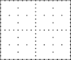
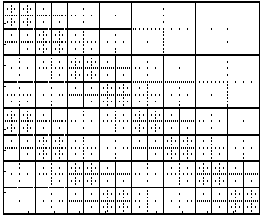
of the index sets one plots the centers of the supports of the active basis
functions. In case of the above simple index sets we get the so-called
regular
sparse grids, see the left Figure below. An
adaptive
sparse grid is shown right. It stems for the numerical solution of
a hyperbolic equation with two diagonal shock fronts in the solution.
|
