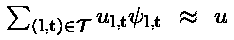
Consider a finite dimensional
approximation to a function
u
:
We want to find an approximation to the
first derivative w.r.t. x
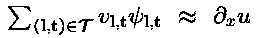
Simple partial derivatives like this are
discretized using finite differences. The main steps are
-
inverse wavelet transform along the
coordinate direction with respect to which we want to differentiate
-
application of the univarite finite difference
scheme
-
wavelet transform with respect to the particular
coordinate direction
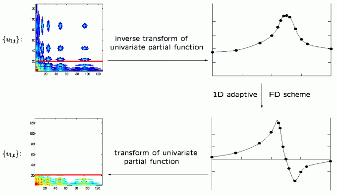
The following figure is a graphical sketch
of this scheme for the 2D case. The squares on the left hand side represent
the wavelet space with a certain arrangement of the indices/wavelet coefficients.
The coloured entries are the coefficients for the indices from T
(the colour corresponds to the magnitude). In each step
just one line (marked by the red bars) of coefficients is read and inverse
transformed. This yields the nodal values of an univariate partial function
on a (non-uniform) grid. To these values the finite difference scheme is
applied. Then, a wavelet transform yields the coefficients of the result.
This repeats for all lines. Vertical lines would be read/written for derivatives
with respect to the y-coordinate direction. An analysis of the resulting
consistency error is given in [6] for regular sparse grids and in
[4] for general adaptive sparse grids.
Another idea for the discretization of
differential operators is collocation. The main adavantages of the finite
difference technique over collocation are:
-
there is no restriction on the smoothness
of the underlying wavelets. This allows to use low order wavelets which
have a small support and are, therefore, algorithmically cheaper than smoother
high order wavelets.
-
even with the same wavelets, the operator
evaluation is much cheaper for the finite difference scheme than for the
collocation method
-
it is quite simple to incorporate special
finite differnce stencils, like ENO/WENO, for differential operators which
require a special treatment for, e.g, stability reasons
|


