Merging of Vortices
The initial configuration are three vortices. Under the influence of the
velocity field they induce, they start to rotate around each other and then to merge.
- domain [0,1]x[0,1] , time: 0.0 ... 80.0 units
- maximum velocity: 0.07 , Re=55000
- time step=5e-3 , finest mesh size=1/2048
The left figure shows the vorticity and the right figure the adaptive grid associated
to the current adaptive basis
Click to see the complete mpeg movie (1.5MB)
Numerical Experiment: 2D Mixing layer
The initial configuration are two flows in the upper and lower half of
[0,1]x[0,1] with opposite sign. The vorticity in the interfacial layer is
randomly perturbated.
Kelvin-Helmholtz instabilities lead to the development of vortices which
in a later stage roll-up and merge. This is a nice example for the tendency
of 2D turbulence to transfer energy from small to large scales. This
leads to a fast decrease of the complexity of the flow and to a decrease
of the number of degrees of freedom required for an accurate numerical simulation.
- domain [0,1]x[0,1] , time: 0.0 ... 80.0 units
- minimum/maximum velocity: -+0.018 , Re=15000
- time step=5e-3 , finest mesh size=1/2048
Click to see the complete mpeg movie (0.8MB)
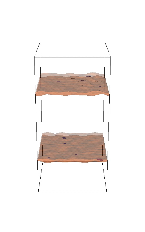
Numerical Experiment: 3D Mixing layer
The initial configuration is the 3D analogue of the 2D mixing layer.
However, due to the 3D character there is an energy transfer from
large to small scales which leads to an increase of the complexity of the flow.
- domain [0,1]x[0,2]x[0,1] , time: 0.0 ... 46.0 units
- minimum/maximum velocity: -+0.018 , Re=3750
- time step=2e-2 , finest mesh size=1/512
- number of DOF from 1 to 2 million
Click to see the complete mpeg movie (1.1MB)